
About REFORCE WebApp
User interface
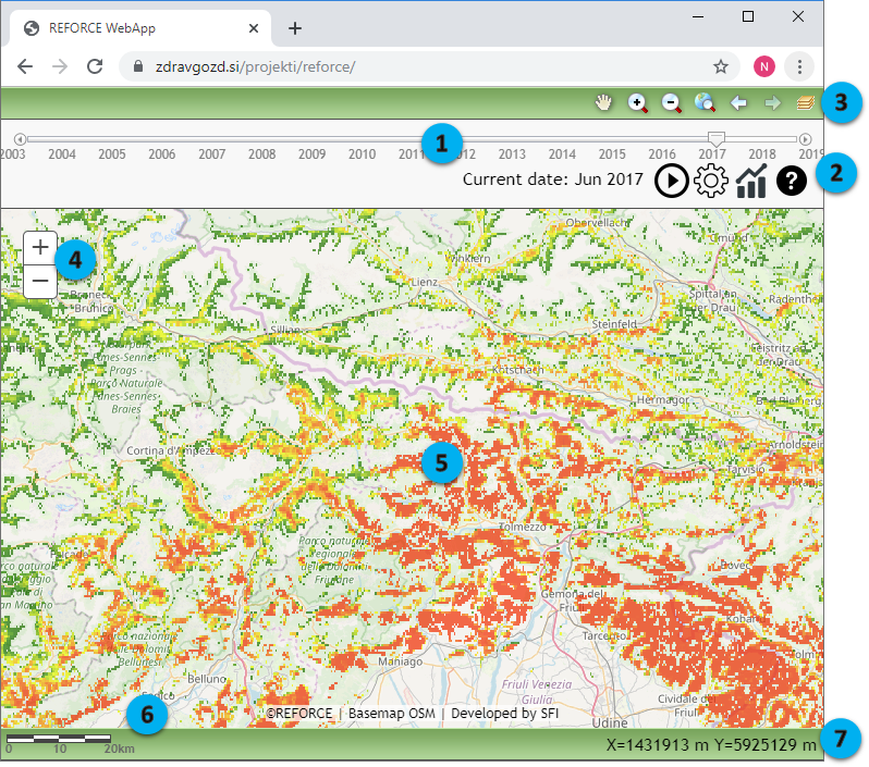
Parts of user interface:
1. Time slider: used to set the time (month and year) when visualizing NDVI data. To the far left there is a button that moves you one step back, and a button to the far right takes one step forward. To move quickly, we use the center arrow on the slider - hold it and move it to the desired position.
2. Tools for animation, analysis, map settings and help. The first button  is for animation management. Pressing the Play button starts the animation of the NDVI data. Press the Stop button
  to end the animation. The speed of the animation is determined in the map settings
  . Tool for Analysis is described below
3. Tools for map management. From left to right: Pan, Zoom in, Zoom out, Zoom to the Alpine region, Previous extent, Next extent, Layers.
4. Zoom in and Zoom out; 5. Map; 6. Scalebar; 7. Coordinates in WGS84 Web Mercator (Auxiliary Sphere) system.
Map layers
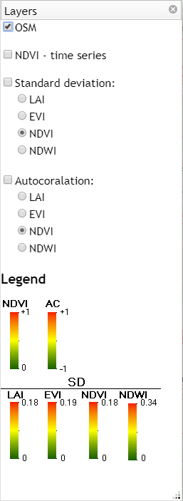
The map has several layers that can be turned on or off:
- OSM – base layer Open Street Map
- NDVI – time series
- Standard deviation (with sublayers LAI, EVI, NDVI, NDWI)
- Autocorrelation (with sublayers LAI, EVI, NDVI, NDWI)
The values for NDVI were normalized to the interval 0 to 1 and similarly for AC to the interval –1 to 1.
Vegetation indices
NDVI – Normalized Difference Vegetation Index
NDVI is based on the normalized difference between the spectral reflectance values in the red and near infrared, i.e. NDVI = (NIR - RED) / (NIR + RED), where NIR is the spectral reflection in the near infrared spectrum and RED is in the red part of the spectrum. NDVI separates green vegetation from other surfaces because chlorophyll absorbs most of the red part of the spectrum and reflects the near-infrared part of the spectrum to a great extent due to structural characteristics of the vegetation. Therefore, high NDVI values relate to high vegetation greenness or biomass. NDVI values range between -1 and +1, those of vegetation usually between 0.2 (sparse vegetation) and 0.8 (dense vegetation).
NDWI – Normalized Difference Water Index
NDWI is used to monitor changes in water content of leaves, using near-infrared (NIR) and short-wave infrared (SWIR) wavelengths. The SWIR reflectance reflects changes in both the vegetation water content and the spongy mesophyll structure of leaves. The NIR reflectance is affected by leaf internal structure and leaf dry matter content, but not by water content. The normalized difference between the NIR and the SWIR removes variations induced by leaf internal structure and leaf dry matter content, improving the accuracy in retrieving the vegetation water content. Interpretation of the values: bright surface with no vegetation or water content has NDWI values between –1 and 0; values from 0 to +1 represent water content.
EVI – Enhanced Vegetation Index
The EVI (Enhanced Vegetation Index) is similar to NDVI, but is enhanced by spectral reflection in the blue part of the spectrum. This enables the correction of the influence of the spectral reflection from the ground and from atmospheric disturbances and reduces saturation of the index over dense stands. It is calculated using the following formula: EVI = 2.5 × [(NIR - RED) / ((NIR) + (6 × RED) - (7.5 × BLUE) + 1)]. NDVI reflects the amount of chlorophyll, and EVI detects structural changes in tree canopies, including leaf area, plant physiognomy, and canopy structure. The difference between NDVI and EVI is that in the case of snow, NDVI is smaller and EVI is larger. EVI values range from -1 to +1, with vegetation typically between 0.2 and 0.8.
LAI – Leaf Area Index
The leaf area index (LAI; without unit) is defined in deciduous trees as single-sided green leaf area per unit area of soil and in conifers as half the total needle area per unit area of soil. We use LAI to predict primary production, evapotranspiration, and as a reference tool for vegetation growth. The LAI interval ranges from 0 (bare ground) to over 10 (dense conifers).
Vegetation dynamics
Two indicators were used to characterize forest dynamics using the remote sensing time series: the standard deviation (sd) and autocorrelation at lag 1 (ac) of the monthly vegetation index anomalies. The standard deviation represents the temporal variability, while the autocorrelation is used as an indicator of temporal slowness of the vegetation response.
Both indicators were derived from Moderate resolution Imaging Spectroradiometer (MODIS) time series (MCD43A4 v6 and MCD15A3H v6 products). Low quality data were masked using the associated quality flags. To homogenize the temporal resolution of the time series and increase their signal to noise ratio (SNR), the time series were aggregated to monthly observations. As seasonal fluctuations do not provide relevant information on the short-term vegetation response to perturbations, the time series were decomposed. The two indicators of forest dynamics were subsequently derived from the anomaly component and pixels with a low forest cover were masked.
Analysis
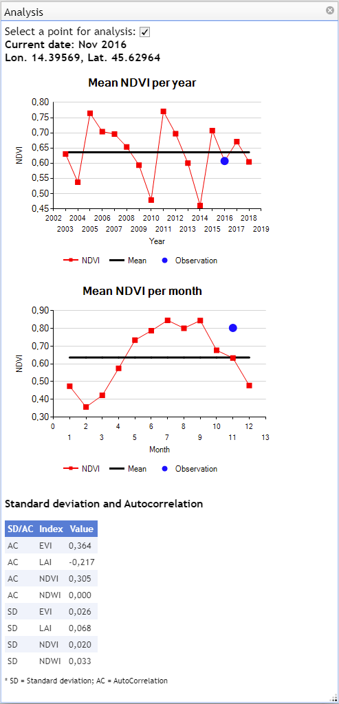
To activate the analysis tool (2), click on the image button with Graph . Select a point on the map, i.e. the raster cell you want to analyze. Wait a few moments for the analysis to complete. The analysis includes two graphs and a table: (1) the first shows annual averages of the NDVI vegetation index of the selected raster cell; (2) the second graph shows the monthly averages of the NDVI vegetation index of the selected raster cell. In both graphs, the black line shows the average of the vegetation index over the whole period, and the blue dots show the values of the selected observation. In the table, the Standard deviation and Autocorrelation values of the vegetation indices are shown for the selected point.
Terms of use
- The REFORCE WebApp is public.
- Its use is free of charge.
- We do not accept any responsibility that may be a direct or indirect consequence of the use of the content from the WebApp.
- Portions of the WebApp may only be copied for non-commercial purposes.
- When using the material from the WebApp you must respect the copyright, i.e. cite the source.
Acknowledgements
The WebApp was developed in the frame of REFORCE project, co-financed by FP7 ERA-NET Sumforest.
Authors
NDVI – time series, SD and AC layers: Wanda De Keersmaecker and Ben Somers, KU Leuven, Belgium
WebApp – Nikica Ogris, Slovenian Forestry Institute, Ljubljana, Slovenia
Technical stuff
Developed with Microsoft Visual Studio 2017 using Microsoft .NET Framework 4.8, ESRI ArcGIS API for JavaScript 3.30, Dojo 1.14.2.
Data stored in ESRI Geodatabase 10.6.1, Microsoft SQL Server 2016, using ESRI ST_RASTER format.
Base map: OSM – Open Street Map